Uncertainty Quantification
Bayesian Sampling
All the figures below are generated using examples/bayesian_sampling/bayesian_sampling.jl.
Model setup

-
Contaminant source (orange rectangle)
-
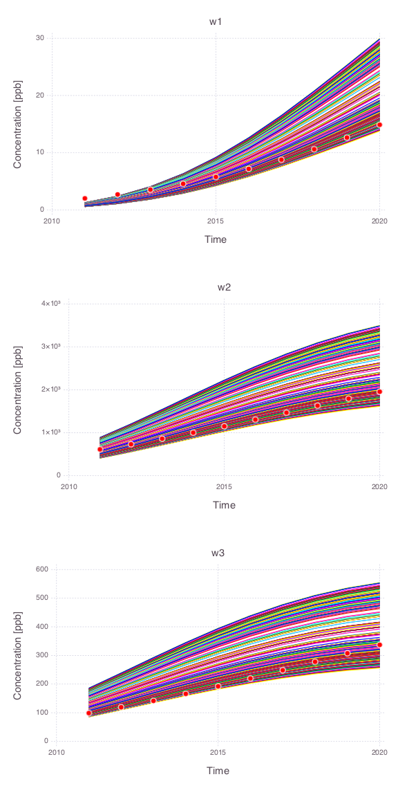
3 monitoring wells
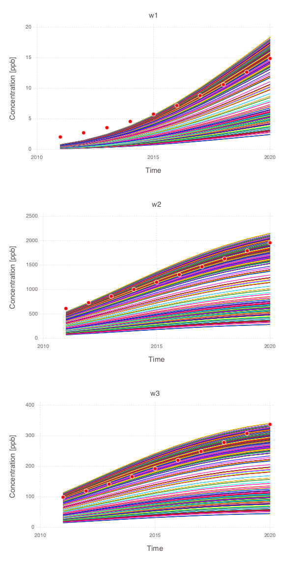
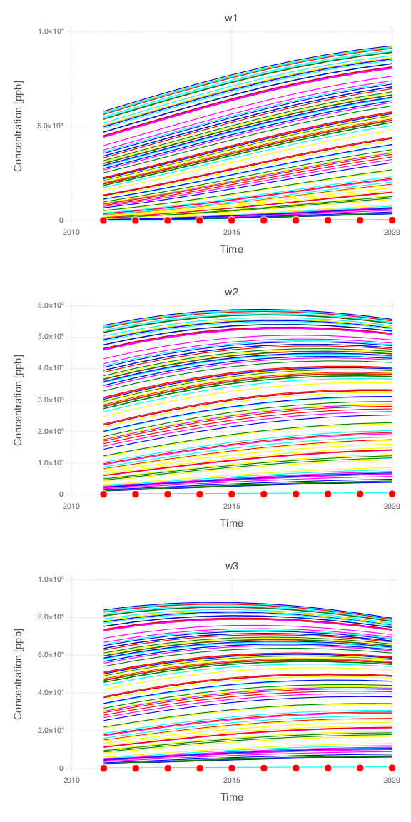
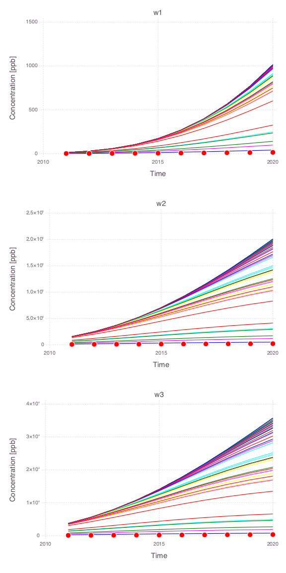
Prior spaghetti plots
Spaghetti plots of 100 model runs representing the prior model prediction uncertainties at the 3 monitoring wells.
Joint spaghetti plots
All model parameters are changed simultaneously within their prior uncertainty ranges.
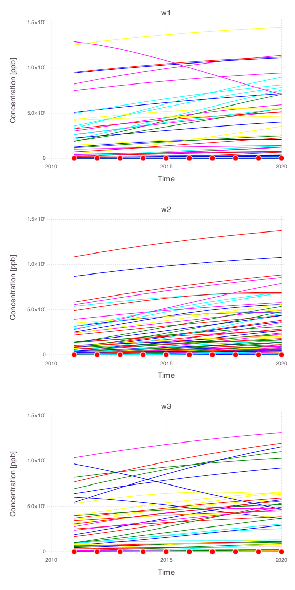
Individual spaghetti plots
A single model parameter is changed at a time.
Source $x$ location
Source $y$ location
Source size along $x$ axis
Source size along $y$ axis
Source release time $t_0$
Source termination time $t_1$
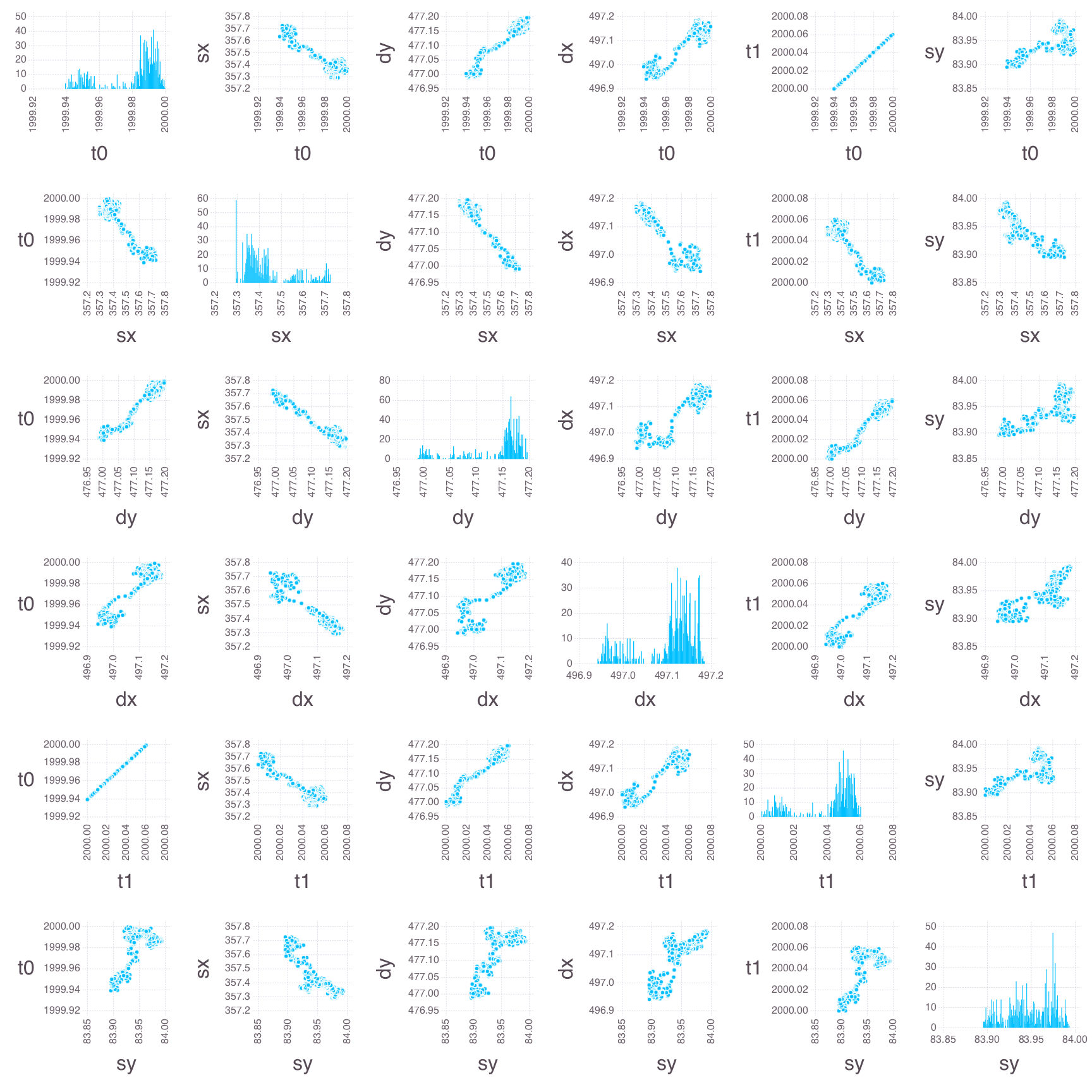
Model calibration match

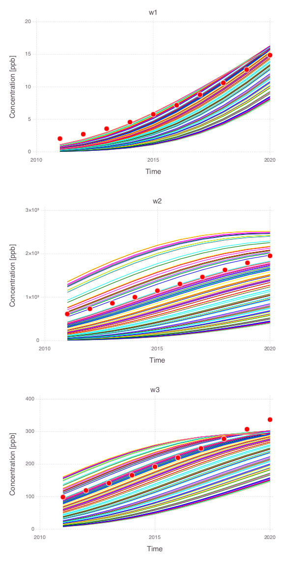
Bayesian sampling results
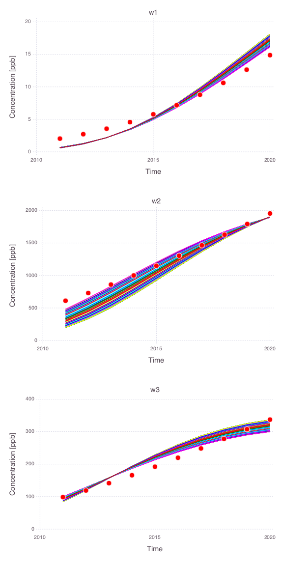
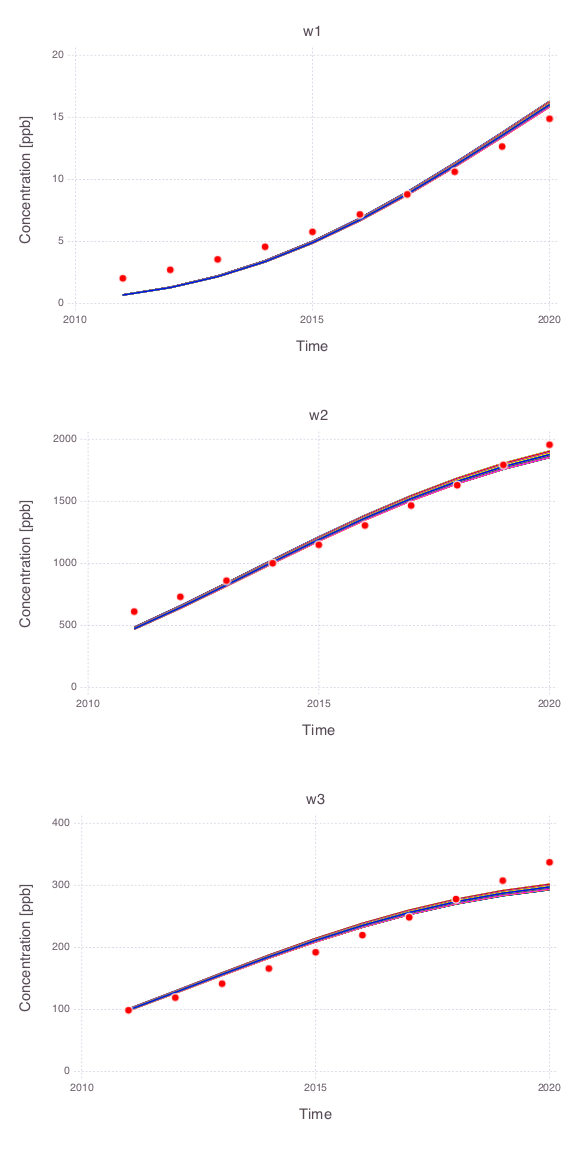
Posterior spaghetti plots
Spaghetti plots of 1000 model predictions representing the posterior model uncertainties at the 3 monitoring wells.
Joint spaghetti plots
All model parameters are changed simultaneously within their prior uncertainty ranges.
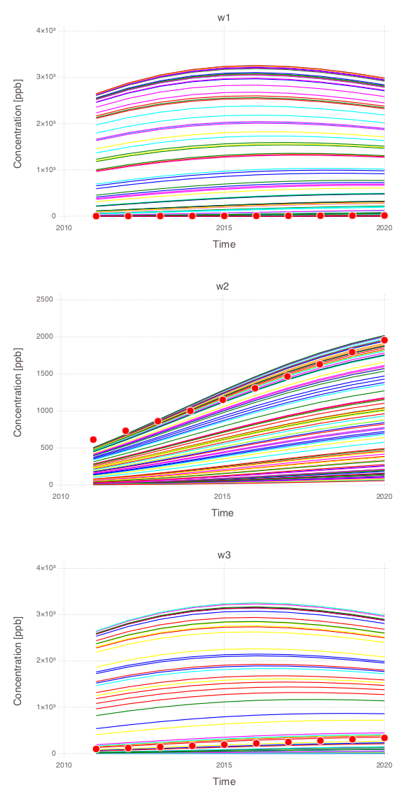
Individual spaghetti plots
A single model parameter is changed at a time.
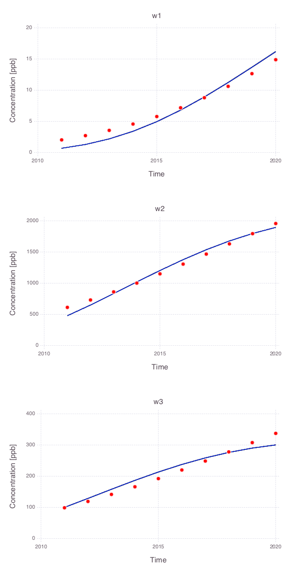
Note that only the posterior uncertainties in the source release time ($t_0$) and the source termination time ($t_1$) are producing large impact in the model predictions.
Source $x$ location (all the 1000 model predictions are overlapping)
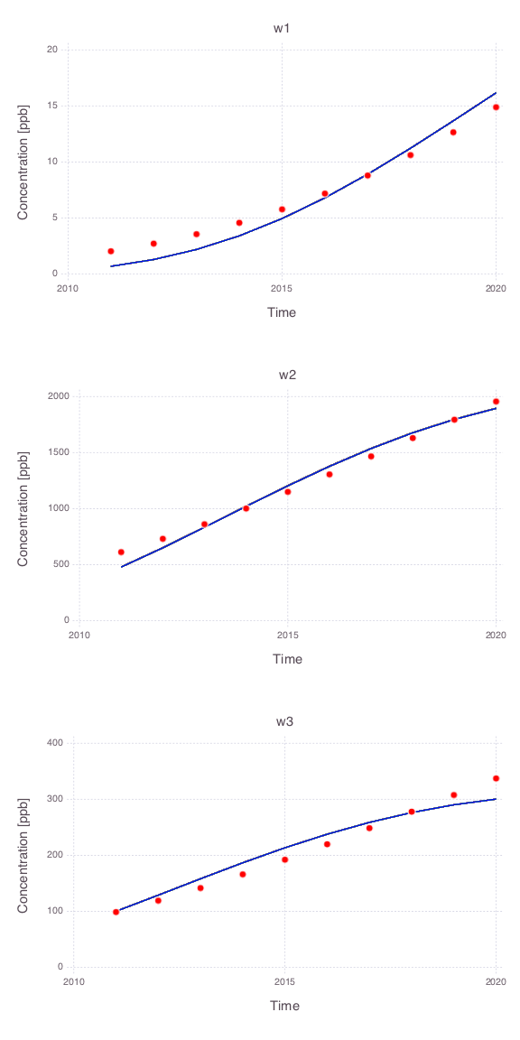
Source $y$ location (all the 1000 model predictions are overlapping
Source size along $x$ axis (all the 1000 model predictions are overlapping
Source size along $y$ axis (all the 1000 model predictions are overlapping
Source release time $t_0$
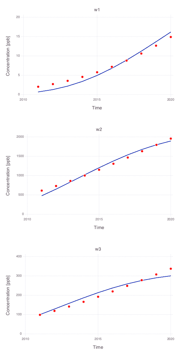
Source termination time $t_1$